Modeling and solving the Traveling Salesman Problem with Python and Pyomo

Feb 2020 8 min read

In this post¹, we will go through one of the most famous Operations Research problem, the Traveling Salesman Problem (TSP). The problem asks the following question:

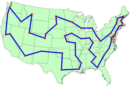
Given a set of cities and the distances between each pair of them, what is the shortest route (tour) that visits each one once and returns to the origin city?

An integer linear programming formulation

The TSP may be formulated as an integer linear programming (ILP) model. In the following, we develop the well known Miller-Tucker-Zemlin (MTZ) formulation. Although it is not the most computationally efficient, it is one of the easiest to code.

Label the cities as $1, …, n$, in which $n$ is the total number of cities and arbitrarily assume 1 as the origin. Define the decisions variables:

$$ x_{ij} = \begin{cases} & 1 \quad \text{ if the route includes a direct link between cities } i \text{ and } j, \\
& 0 \quad \text{ otherwise}. \end{cases} $$

In addition, for each city $i = 1, 2, …, n$, let $u_i \in \mathbb{R}^+$ be an auxiliary variable and let $c_{ij}$ be the distance between cities $i$ and $j$. Then, the MTZ formulation to the TSP is the following: $$ \begin{align} \text{min} \quad & \sum_{i = 1}^{n} \sum_{j = 1, j \neq i}^{n} c_{ij} x_{ij}, \\
\text{subject to} \\
& \sum_{i=1, i \neq j}^{n} x_{ij} = 1, \quad j=1,2,…,n,\\
& \sum_{j=1, j \neq i}^{n} x_{ij} = 1, \quad i=1,2,…,n,\\
& u_i - u_j + n x_{ij} \leq n-1, \quad 2 \leq i \neq j \leq n, \\
& x_{ij} \in \{0,1\} \quad i, j =1,2,…,n, \quad i \neq j, \\
& u_i \in \mathbb{R}^+ \quad i=1,2,…,n. \\
\end{align} $$

In the formulation above, notice that the first set of equalities requires that each city is arrived at from exactly one other city, and the second set of equalities requires that from each city there is a departure to exactly one next city. Notice that these constraints do not guarantee the formation of a single tour encompassing all cities, allowing the formation of subtours. In order to exclude subtour solutions, the third constraint set is needed. These are known as the MTZ subtour elimination constraints.

Introducing Pyomo

To solve the TSP we will make use of Pyomo, which is a Python-based open-source optimization modeling language. If you had experience with any programing language (especially Python), modeling and solving a problem with Pyomo will be a simple task.

Pyomo allows you to choose among a variety of integer linear programming solvers, both open-source and commercial. For this post, we will make use of the CPLEX IBM Solver, to solve the MTZ formulation of the TSP. Feel free to use any other solver for ILP.

Data reading

The first step is to enter the data. This means to provide a distance matrix (or cost matrix), which gives the pairwise distances between cities.

For pedagogical and pratical purposes, we will use a cost matrix for $n = 17$ cities ( click here to download the file ). The file can be read in Python in the following way:

file = open('17.txt')
lines = file.readlines()
file.close()

for i in range(len(lines)):
    aux = lines[i][:-1].split('\t')
    aux = [int(i) for i in aux if i!= '']
    cost_matrix.append(aux)

n = len(cost_matrix)

The variables cost_matrix and n contain the cost matrix and the number of cities, respectively. Now we will be able to call these elements when defining constraints.

Model building

To use Pyomo and solve the problem we need to make a single import:

import pyomo.environ as pyEnv

Now we can initialize the model:

#Model
model = pyEnv.ConcreteModel()

#Indexes for the cities
model.M = pyEnv.RangeSet(n)                
model.N = pyEnv.RangeSet(n)

#Index for the dummy variable u
model.U = pyEnv.RangeSet(2,n)

in which

ConcreteModel() creates the model;
RangeSet(n) creates an index from 1 to n;
RangeSet(2,n) creates an index from 2 to n.

Decision variables

The decision variables are declared in the following way:

#Decision variables xij
model.x = pyEnv.Var(model.N,model.M, within=pyEnv.Binary)

#Dummy variable ui
model.u = pyEnv.Var(model.N, within=pyEnv.NonNegativeIntegers,bounds=(0,n-1))

in which

Var(model.N,model.M, within=pyEnv.Binary) creates $n$ binary decision variables of size $m$;
Var(model.N, within=pyEnv.NonNegativeIntegers,bounds=(0,n-1)) creates $n$ non-negative integer decision variables that can only assume values between 0 and $n-1$.

Cost matrix

Next, we must provide the model with the cost matrix:

#Cost Matrix cij
model.c = pyEnv.Param(model.N, model.M,initialize=lambda model, i, j: cost_matrix[i-1][j-1])

in which Param(modelo.N, model.M,initialize=lambda model, i, j: cost_matrix[i-1][j-1]) provides a $n \times m$ parameter to the model using a lambda function.

Objective function

After defining all the variables and provide the parameters, we are able to declare the objective function:

def obj_func(model):
    return sum(model.x[i,j] * model.c[i,j] for i in model.N for j in model.M)

model.objective = pyEnv.Objective(rule=obj_func,sense=pyEnv.minimize)

First we create a Python function that returns our objective function. Notice that we used the list comprehension technique. If you’re not familiar with it, this page gives a pretty good tutorial.

Objective(rule=obj_func,sense=pyEnv.minimize) creates the objective function of the model and sets its optimization direction (maximize or minimize). In the TSP we want to minimize total cost, so that we set sense=pyEnv.minimize.

Constraints

Constraints are declared in a way very similar to the objective function. The first constraint set, which ensures that each city is arrived at from exactly one other city can be formulated in the following way:

def rule_const1(model,M):
    return sum(model.x[i,M] for i in model.N if i!=M ) == 1

model.const1 = pyEnv.Constraint(model.M,rule=rule_const1)

in which Constraint(model.M,rule=rule_const1) creates $m$ constraints defined by rule_const1.

The second constraint set, which ensures that from each city there is a departure to exactly one next city can be formulated by:

def rule_const2(model,N):
    return sum(model.x[N,j] for j in model.M if j!=N) == 1

model.rest2 = pyEnv.Constraint(model.N,rule=rule_const2)

in which Constraint(model.N,rule=rule_const2)creates $n$ constraints defined by rule_const2.

The third and last constraint set correspond to the MTZ subtour elimination constraints:

def rule_const3(model,i,j):
    if i!=j: 
        return model.u[i] - model.u[j] + model.x[i,j] * n <= n-1
    else:
        #Yeah, this else doesn't say anything
        return model.u[i] - model.u[i] == 0 
    
model.rest3 = pyEnv.Constraint(model.U,model.N,rule=rule_const3)

in which Constraint(model.U,Model.N,rule=rule_const3) creates $u \times n$ constraints defined by the rule_const3.

A rule type function must provide a Pyomo object, so that’s why we had to write a weird else condition.

Finally, we can print the entire model in the screen by calling:

#Prints the entire model
model.pprint()

in which pprint() prints de entire model (it might not be a good idea if the model is too big). Alternatively, we can use pprint(filename=’file.txt’) to print the model in a specific file.

Solving the model

In order to solve the model, we must have a previously installed solver, since Pyomo is just a modeling language. We will use the widely known commercial solver IBM CPLEX, but you can use many other commercial and non-commercial solvers, such as Gurobi, GLPK, CBC, etc.

The following code creates an instance of the solver and then solves the model:

#Solves
solver = pyEnv.SolverFactory('cplex')
result = solver.solve(model,tee = False)

#Prints the results
print(result)

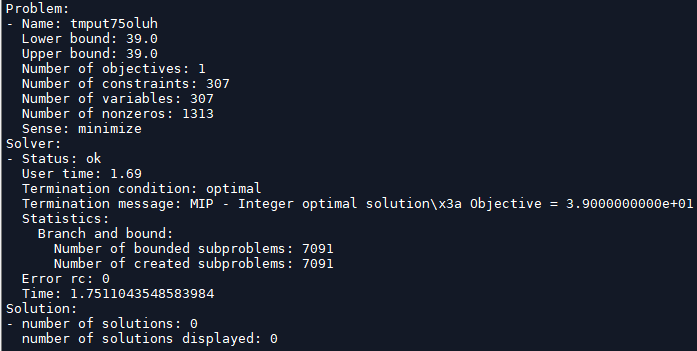
in which SolverFactory(‘cplex’) initializes the solver instance and solve(model, tee= False) solves the model. Setting tee = False disables the solver’s log messages. In order to enable it, just set tee= True. Figure below shows the results returned by the solver:

In order see the values of the decision variables, we can do as the following:

l = list(model.x.keys())
for i in l:
    if model.x[i]() != 0:
        print(i,'--', model.x[i]())

The figure below shows only the variables for which $x_{ij} = 1$.

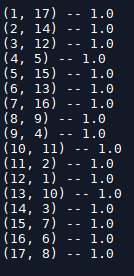
Variables for which $x_{ij} = 1$ in the optimal tour.

Then, the optimal tour starting from city 1 is $$ \begin{align} & 1 \to 17 \to 8 \to 9 \to 4 \to 5 \to 15 \to 7 \to 16 \to 6 \to \\
& \to 13 \to 10 \to 11 \to 2 \to 14 \to 3 \to 12 \to 1 \end{align} $$

In practice

The TSP is a widely studied prototypical NP-hard problem. The number of possible tours increases as a factorial of the number of cities. The MTZ-based formulation cannot obtain optimal solutions to large instances in acceptable wall clock times, since its linear relaxation is very weak. There are alternative approaches which can obtain optimal or very good solutions to large instances. Concorde is an exact algorithm based on Dantzig's cutting plane method which has obtained an optimal tour for an instance with 85900 cities. Alternatively, very good tours may be obtained by using heuristics such as LKH or simulated annealing.

Therefore, the TSP is considered a solved problem in practice. However, the more general class of vehicle routing problems (VRP), which include other constraints absent in the classical TSP, is far from being satisfactorily solved. To name a few constraints found in real problems from the many possible: multiple vehicles with limited capacity, multiple depots, time windows, fractional loads, stochastic demands and heterougenous fleets. The combination of these constraints give rise to different problems with varying degrees of difficulty.

Extras

To find more examples of Pyomo you can go to their GitHub page. In addition, you can find a Pyomo manual in Portuguese in my own GitHub page.

This post is an adaptation of an article originally published in Medium. ↩︎