A deep reinforcement learning approach for the asynchronous dynamic vehicle dispatching problem
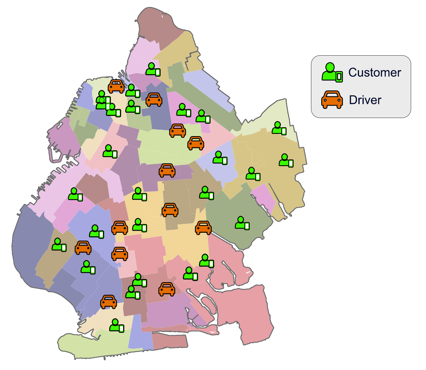
Imagine you manage a fleet of taxis in a large city. Ride requests pop up at unpredictable times and places, and drivers become available whenever they finish a trip. Every time one of these events happens, you have to decide — right now — which vehicle serves which request. Wait too long and passengers cancel; assign carelessly and you leave money and service quality on the table.
This is the dynamic vehicle dispatching problem (DVDP): assigning vehicles to requests that arise stochastically over time and space. It shows up in taxi and ride-hailing services, food delivery, truckload transportation, open-pit mining, and emergency systems such as police patrol and ambulance dispatching.
The DVDP is fundamentally different from classical vehicle routing. In routing problems, demand and resources are generally known in advance, and the goal is to compute an optimal plan (e.g., the best set of routes). In the DVDP, a control agent must assign vehicles to requests in real time, based on the current state of the system. It is best understood as an optimal control problem — precisely the kind of setting where reinforcement learning shines.
Synchronous vs. asynchronous dispatching
Dynamic dispatching can be done in two modes:
- Synchronous mode: assignments happen at fixed time intervals. At each decision epoch, a central agent collects all pending requests and available vehicles and solves a combinatorial matching problem (typically a linear assignment problem).
- Asynchronous mode: dispatching is triggered immediately whenever a request arrives or a vehicle becomes idle. There is no need to wait for the next decision cycle.
Most of the literature studies the synchronous mode, yet the asynchronous mode has real practical advantages. In police patrol or ambulance management, waiting for a “batch” of incidents to form is socially unacceptable — a vehicle must go as fast as possible. Asynchronous dispatching also enables distributed rather than centralized decision-making, and it dramatically shrinks the decision space: instead of choosing among all possible matchings (a combinatorial explosion), the agent only has to pick a single vehicle for a request, or a single request for a vehicle.
Despite these advantages, the asynchronous DVDP remains largely unexplored. This post summarizes our approach to formulating and solving it.
Formulating the problem as a semi-Markov decision process
The defining feature of the asynchronous DVDP is that decision epochs occur at random points in continuous time. Two events trigger a decision:
- a “new call” event, when a new request is communicated to the agent, and
- a “free vehicle” event, when a vehicle finishes serving a request.

Because these events happen stochastically, the time intervals between successive decisions are themselves random. This is exactly what a semi-Markov decision process (SMDP) captures — a generalization of the Markov decision process (MDP) that allows decision epochs to be separated by random time intervals.
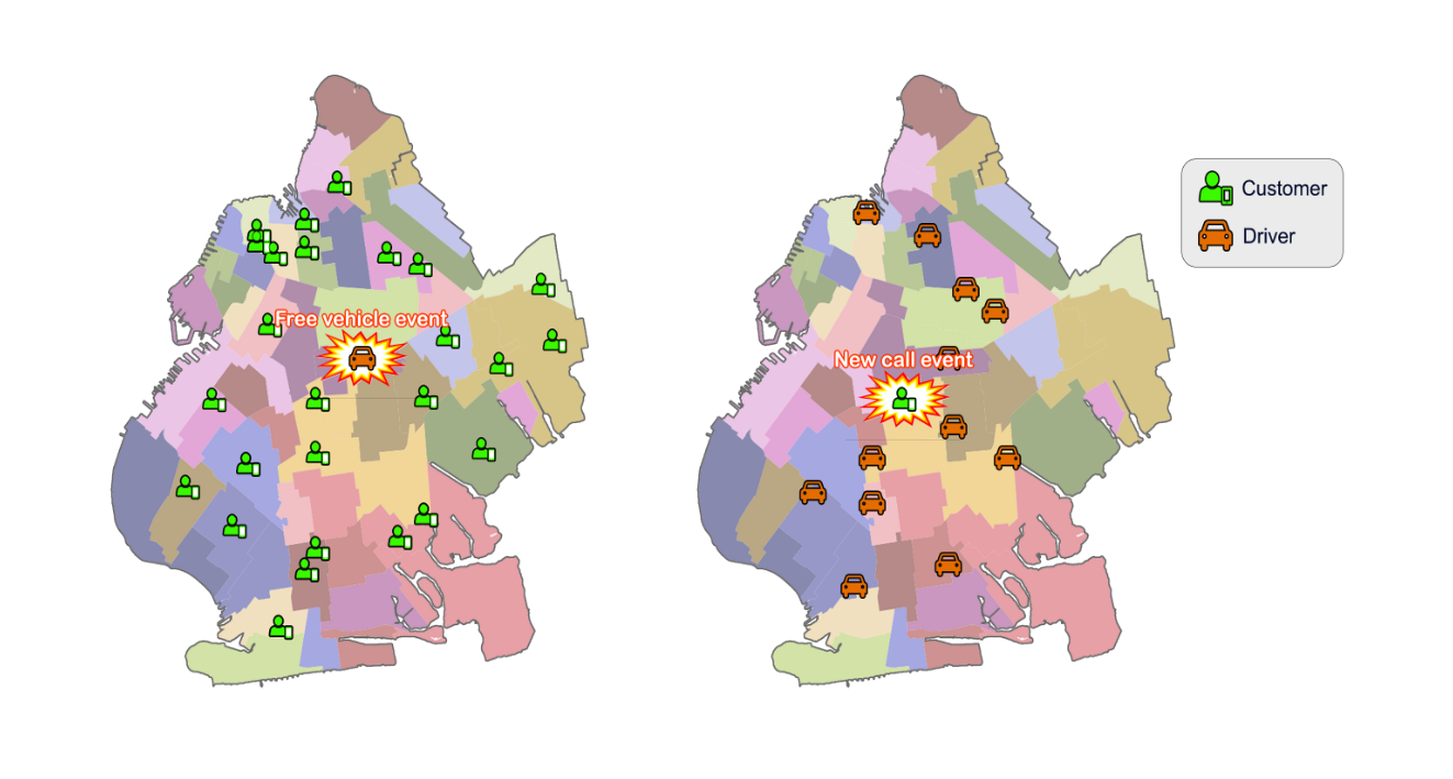
Another key characteristic is that the set of feasible decisions $\mathcal{A}(s)$ depends on which event fired:
- On a free vehicle event, the agent picks which waiting request to assign to the newly available vehicle. The size of $\mathcal{A}(s)$ grows linearly with the number of pending requests (and is empty if none are waiting).
- On a new call event, the agent picks which free vehicle to assign to the incoming request. The size of $\mathcal{A}(s)$ grows linearly with the number of free vehicles (and is empty if none are available).
We seek a policy $\pi$ that maximizes the expected discounted reward stream over an infinite horizon:
$$ v^\star(s) = \max_{\pi \in \Pi} \lim_{N \to \infty} \mathbb{E} \Bigg[ \sum_{k=0}^{N-1} \int_{T_{k}}^{T_{k+1}} e^{-\beta t} r(S_k, \pi(S_k)) dt \Bigg| S_0 = s \Bigg], \quad \forall s \in \mathcal{S}.$$
Notice that the reward is integrated over the random intervals between decision epochs $T_k$ and $T_{k+1}$, and $e^{-\beta t}$ is the continuous-time analog of the usual discrete discount factor $\gamma$ (with $e^{-\beta} = \gamma$). The corresponding Bellman equation for the discounted SMDP is:
$$ v^\star(s) = \max_{a \in \mathcal{A}(s)} \Big\lbrace \bar{r}(s,a) + \mathbb{E}\big[e^{-\beta \tau} v^\star(S’)\big] \Big\rbrace, \quad \forall s \in \mathcal{S} $$
where $\bar{r}(s,a)$ is the expected reward accumulated between two consecutive decision epochs. The only real difference from the ordinary MDP Bellman equation is the random interval $\tau$ that appears in the discount term.
Why not just solve it exactly? Exact dynamic programming (value or policy iteration) requires enumerating the entire state space. But a state must, at minimum, encode the locations of every vehicle and every request — so the state space grows exponentially with fleet and demand size. On top of that, the complex dynamics make it impossible to write a closed-form expression for the transition probabilities. Exact methods are hopeless for realistic instances, which motivates a simulation-plus-learning approach.
The synchronous case as a special case
Synchronous dispatching can be seen as a constrained SMDP in which decision epochs are forced to occur at fixed intervals — that is, an ordinary MDP. Its Bellman equation is simply
$$ v^\star(s) = \max_{a \in \mathcal{A}(s)} \Big\lbrace r(s, a) + \gamma \mathbb{E}[v^\star(s’)] \Big\rbrace, \quad \forall s \in \mathcal{S}.$$
The catch is the action set: in synchronous mode, $\mathcal{A}(s)$ contains all feasible matchings between vehicles and requests, so choosing the best action means solving an integer nonlinear program at every step. To make this tractable, authors usually relax the global Q-function into a sum of per-pair terms $\tilde{q}_{ij}$ and solve a linear assignment problem instead:
$$ \begin{align} \max \quad & \sum_{i=1}^n \sum_{j=1}^n \tilde{q}_{ij}, x_{ij} \\ \text{s.t.} \quad & \sum_{j=1}^n x_{ij} = 1, \quad i \in \mathcal{I} \\ & \sum_{i=1}^n x_{ij} = 1, \quad j \in \mathcal{J} \\ & x_{ij} \in {0,1}, \quad (i,j) \in \mathcal{I} \times \mathcal{J}. \end{align} $$
This relaxation makes computation tractable, but it decomposes the global value into independent driver–request contributions, ignoring their interactions and producing decisions from an individual rather than a global perspective. The fixed intervals also add latency: a passenger rejected in one cycle must wait for the next. Asynchronous dispatching sidesteps both issues — a new vehicle can be proposed the instant a rejection happens.
Our solution: deep RL + discrete-event simulation
Like most modern RL methods, we work with Q-functions (action-value functions). The optimal Q-function satisfies the SMDP Bellman equation
$$ q^\star(s,a) = \bar{r}(s,a) + \mathbb{E}\Big[ e^{-\beta \tau} \max_{a’ \in \mathcal{A}(s’)} q^\star(s’,a’)\Big] $$
and, once known, an optimal policy is obtained by acting greedily: $\pi^\star(s) \in \arg\max_{a \in \mathcal{A}(s)} q^\star(s,a)$. The advantage of Q-functions is that they are **model-free** — we don't need an explicit probability model of the environment's dynamics to act.
Two specialized agents
We initially tried a single agent handling both event types, but training was unstable. Splitting the problem into two specialized agents worked far better:
- the
NewCallAgent, which acts on new-call events (from the passengers’ perspective), and - the
FreeVehicleAgent, which acts on free-vehicle events (from the drivers’ perspective).
Each agent focuses on its own decision space and learns better decisions for its side of the problem.

Because the state space is enormous, we use neural networks as function approximators for the Q-function. Whenever a decision event occurs during the simulation, the corresponding agent builds a feature vector $\phi(s,a)$ for each feasible action, feeds it through its network to get $\hat{q}(s,a)$, and picks the action with the highest estimated Q-value. Since the action set grows only linearly, evaluating all candidates is fast — well within the time budget of an online system.

Learning from simulated experience
Sample trajectories are generated by a discrete-event simulator. As the simulation runs, each transition is stored in an experience buffer as a tuple
$$ (s, a, r, s’, \tau) $$
where $s$ is the current state, $a$ the decision, $r$ the reward, $s'$ the next state, and $\tau$ the realized transition time. We train the networks with the double deep Q-learning algorithm, which uses two networks (A and B) to reduce the overestimation bias of standard Q-learning. Given a sampled transition, network A is updated toward the target
$$ Y^{\text{DoubleQ}} = r + e^{-\beta \tau}, q\Bigg(s’, \arg\max_{a’ \in \mathcal{A}(s’)} q(s’, a’; \boldsymbol{\theta}^{\text{A}}_t);\ \boldsymbol{\theta}^{\text{B}}_t\Bigg) $$
with network B updated symmetrically. Learning kicks in once the buffer has accumulated enough initial transitions (gathered under a random policy), and both agents are trained concurrently as the simulation unfolds.
Case study: taxi fleet management in New York City
We validated the approach on a realistic taxi fleet management scenario using New York City Taxi and Limousine Commission trip records. We restricted the study to trips within the Brooklyn borough completed via Uber or Lyft, using January 2022 data for training and February 2022 data — completely isolated to prevent leakage — for testing. All distances used the Manhattan (L1) metric.

The trace-driven discrete-event simulator was built with SimPy . To increase realism, we modeled assignment rejections: each driver's rejection probability is drawn from a beta distribution, and each passenger's waiting tolerance from a gamma distribution (so requests waiting too long get cancelled).
State and action features
Each state–action pair $(s,a)$ is mapped to a feature vector $\phi(s,a)$ combining information about the vehicle, the request, and the broader context:
| Index | Type | Feature description |
|---|---|---|
| 1 | vehicle | (x, y) coordinates of the vehicle's current location |
| 2 | vehicle | (x, y) coordinates of the vehicle's destination |
| 3 | vehicle | Time to finish the current service |
| 4 | vehicle | Cancellation probability |
| 5 | vehicle | Vehicle status (busy or idle) |
| 6 | request | (x, y) coordinates of the request origin |
| 7 | request | (x, y) coordinates of the request destination |
| 8 | request | Time the request arrived in the system |
| 9 | context | #vehicles / #requests ratio in the last 15 minutes |
| 10 | context | Week cyclical feature: $\sin(2\pi, m / 10080)$ |
| 11 | context | Week cyclical feature: $\cos(2\pi, m / 10080)$ |
Here $m$ is the minute within the week (10080 minutes = 1 week), so the cyclical features let the model capture weekly demand patterns.
Designing the reward function
Getting the reward right was crucial. Rewarding only short waiting times backfired: agents learned to serve the newest requests and let old ones languish until cancellation. Our final reward starts from a term proportional to the ride duration, plus a fixed bonus:
$$ r_d = t_d + b $$
where $t_d$ is the estimated origin-to-destination travel time. Longer rides are more desirable (higher earnings), while the constant $b$ acts as a fixed per-ride reward that encourages higher service rates. Tuning $b$ balances “many short trips” against “fewer long trips.” Finally, since the total service time $t_s$ is random, we discount the reward over that duration:
$$ r = \dfrac{r_d}{t_s} + \gamma \dfrac{r_d}{t_s} + \cdots + \gamma^{t_s-1} \dfrac{r_d}{t_s} = \dfrac{r_d(\gamma^{t_s} - 1)}{t_s(\gamma - 1)} $$
so that assignments with the same immediate reward but different durations are valued differently.
Results
We compared the learned policy (labeled DQN) against four asynchronous heuristics — Nearest Neighbor (NN), First-In-First-Out (FIFO), Last-In-First-Out (LIFO), and Random — and two synchronous batch policies solving a linear assignment problem every 15 seconds with the Jonker–Volgenant algorithm:
- BWO — batch without previous waiting time (minimizes vehicle-to-origin travel time only), and
- BW — batch with previous waiting time (minimizes waiting + travel time).
We evaluated four supply-to-demand regimes — “very easy,” “easy,” “average,” and “hard” — corresponding to fleet-to-demand ratios of 3%, 2%, 1%, and 0.5%. Three metrics were tracked: average delay (time from request to pickup), cancellation rate, and total service time (a proxy for driver revenue).
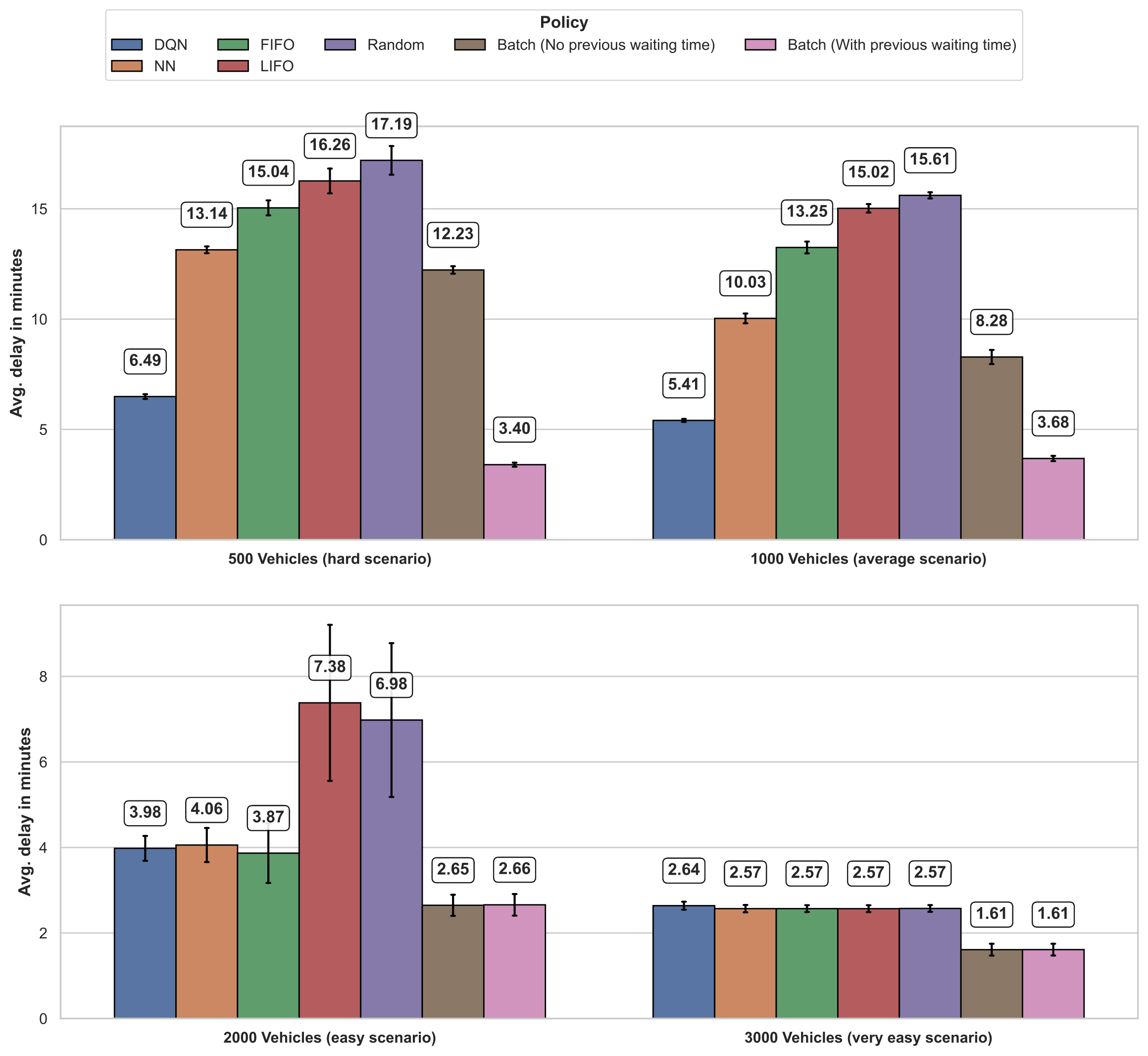
Average delay. Among the asynchronous policies, DQN reduced average delay by 50.6% relative to the second-best (NN) in the hard scenario. The synchronous BW policy achieved the lowest delay overall (3.4 min vs. 6.49 min for DQN in the hard scenario), thanks to its “wait-and-see” strategy — but, as we'll see, that comes at a cost.

Cancellation rate. In the hard and average scenarios, DQN achieved the lowest cancellation rate of all policies — an 18.4% reduction over the second-best (BWO) in the hard scenario. Because asynchronous policies assign vehicles as soon as possible, they avoid the cancellations that the batch policies’ waiting strategy induces. This reveals a genuine trade-off: BW wins on delay but favors short-waiting requests, letting others linger until they cancel.
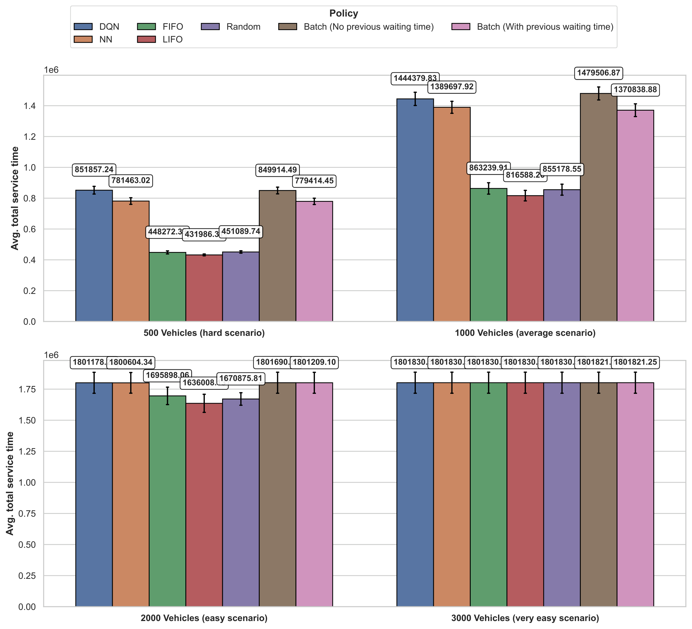
Total service time. DQN and BWO delivered the highest total service times (driver revenue) in the hard scenario, with no statistically significant difference between them; differences were negligible in the easier scenarios.

Finally, the DQN policy maintains the smallest pool of waiting requests throughout most of the day, especially during peak hours — a direct consequence of its assign-as-soon-as-possible nature.
Overall, the asynchronous learning-based DQN policy strikes an effective balance between service efficiency and reliability, performing especially well in the resource-constrained scenarios that matter most in practice.
Conclusion
We formulated the asynchronous dynamic vehicle dispatching problem as a semi-Markov decision process and solved it by combining discrete-event simulation with deep reinforcement learning, using two specialized agents trained via double deep Q-learning. On real NYC taxi data, the learned policy achieved up to a 50.6% reduction in average passenger delay and an 18.4% reduction in cancellation rates compared with other asynchronous policies, while maintaining comparable total service times.
The framework provides a scalable, adaptable foundation for real-time fleet management under uncertainty. Future directions include multi-agent settings, integrating demand forecasting, and improving policy transferability across operational contexts.
This work was financed in part by CNPq (Grant No. 407466/2021-5) and by NVIDIA Corporation through the GPU Grant Program.
References
[1] Cordeiro, F. E. A.; Pitombeira-Neto, A. R. A deep reinforcement learning approach for the asynchronous dynamic vehicle dispatching problem. Artificial Intelligence for Transportation, 3–4, 100038, 2025. https://doi.org/10.1016/j.ait.2025.100038
[2] Powell, W. B. A stochastic formulation of the dynamic assignment problem, with an application to truckload motor carriers. Transportation Science, 30(3), 195–219, 1996.
[3] Xu, Z. et al. Large-scale order dispatch in on-demand ride-hailing platforms: A learning and planning approach. Proceedings of the 24th ACM SIGKDD, 2018.
[4] Puterman, M. L. Markov Decision Processes: Discrete Stochastic Dynamic Programming. John Wiley & Sons, 2014.
[5] van Hasselt, H.; Guez, A.; Silver, D. Deep reinforcement learning with double Q-learning. Proceedings of the AAAI Conference on Artificial Intelligence, 2016.
Cite this paper
Cordeiro, F. E. A., & Pitombeira-Neto, A. R. (2025). A deep reinforcement learning approach for the asynchronous dynamic vehicle dispatching problem. Artificial Intelligence for Transportation, 3–4, 100038. https://doi.org/10.1016/j.ait.2025.100038
@article{cordeiro2025deep,
  title     = {A deep reinforcement learning approach for the asynchronous dynamic vehicle dispatching problem},
  author    = {Cordeiro, Francisco Edyvalberty A. and Pitombeira-Neto, Anselmo R.},
  journal   = {Artificial Intelligence for Transportation},
  volume    = {3--4},
  pages     = {100038},
  year      = {2025},
  issn      = {3050-8606},
  doi       = {10.1016/j.ait.2025.100038},
  publisher = {Elsevier}
}

Anselmo R. Pitombeira Neto
Associate Professor
Associate Professor at UFC and leader of the OPL. His research interests include applications of artificial intelligence and operations research to problems in production, logistics, transportation, energy and health.